Part 1

This article tries to lay a foundational understanding for Bayes theorem. Especially what does it actually mean when you multiply two probabilities. This stems from Bayes theorem and we will explore it with an example.

Note: We will use the wonderful example provided in Quora, here and try to elaborate visually.

Problem: Given the weather forecast(WF) is rain, what is probability that it would actually rain in my area?

Assumptions: Out of 100 days rained, WF predicted correctly 90% of the time that it rained. Out of 100 days dry, WF predicted correctly 80% of the time, that it would be dry. In my area, out of 100 days, 10 days it would rain and 90 days would be dry.

We could visualize them as below. Visualization is the key here in this article to understand, why the heck we "multiply" probabilities.

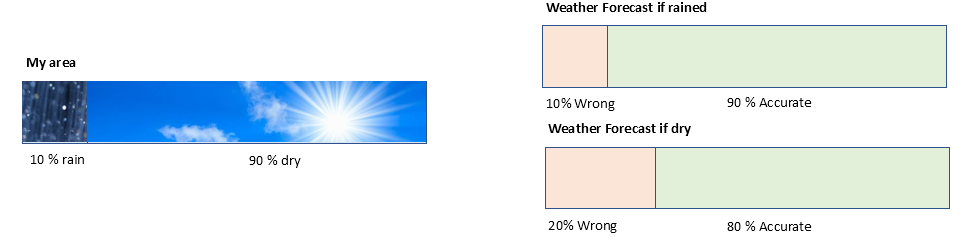
If we try to apply WF for both rain and dry cases in my area, it would be something like this (not drawn to scale).

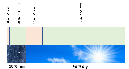
For 10% of time raining in my area, WF would be 90% accurate to predict that it would rain. In other words, out of 10% days raining, WF would be 90% of the time, correctly would predict as rain.

90% out of 10% days raining is 90%(10%) = (0.9)(0.1) = 0.09 or 9%

Thus, 9% of the time in my area, its rains and WF would predict correctly as rain. 

That's it. This is how the multiplication is evolving out of our logic. Its not yet over.

From Figure 2, again, for 90% of time being dry in my area, WF would be wrong 20% of the time. That is WF would be predicting as rain, but it would be dry here. In other words, out of 90% days being dry, WF would be 20% of the time wrongly predicting as rain.

20% out of 90% days being dry is = (0.2)(0.9) = 0.18 or 18%

Thus, 18% of the time in my area, its dry, and WF would wrongly predict as rain.

In terms of probability, if

$$ p(R_{\text{Act}})=\text{Probability of raining in my area} \ p(D_{\text{Act}})=\text{Probability of dryness in my area} \ p(R_{\text{WF}})=\text{Probability of WF as rain generally} \ p(D_{\text{WF}})=\text{Probability of WF as dry generally}\p(R_{\text{Act}} \cap R_{\text{WF}}) = \text{Probability that it rains and WF also predicts rain} \ p(D_{\text{Act}} \cap R_{\text{WF}}) = \text{Probability that it is dry and WF predicts rain} $$

Then what we inferred in words above, can be expressed as,

$$ p(R_{\text{Act}} \cap R_{\text{WF}}) = (0.1)(0.9) = 0.09 \ p(D_{\text{Act}} \cap R_{\text{WF}}) = (0.9)(0.2) = 0.18 \tag{1}
$$

Putting it another way, out of 100 days in my area, {9 days it rains and WF also predicts as rain} and {18 days its dry and WF predicts as rain}.

Let us stop a moment and recall basic probability now:

$ \text {Probability of favourable outcome} = \frac{\text {No of favourable outcomes}}{\text {Total no of possible outcomes}} $

In our case,

$$ \text {Total no of days its rain given WF says rain} = 9
\ \text {Total no of days its dry given WF says rain} = 18 \ \text {Total no of days either rain or dry given WF says rain} = 9 + 18 = 27 $$

Deploying that,

$$
p(\text {actual rain given WF says rain}) = \frac{9}{9+18} = \frac{1}{3} = 0.33\ p(\text {actually dry given WF says rain}) = \frac{18}{9+18} = \frac{2}{3} = 0.66 $$

We have a math notation for LHS..

$$ p(R_{\text{Act}} \mid R_{\text{WF}}) = 0.33\ p(D_{\text{Act}} \mid R_{\text{WF}}) = 0.66 \tag{2} $$

Combining equations (1) and (2), we could thus see,

$$ p(R_{\text{Act}} \mid R_{\text{WF}}) = \frac{p(R_{\text{Act}} \cap R_{\text{WF}})}{p(R_{\text{Act}} \cap R_{\text{WF}}) + p(D_{\text{Act}} \cap R_{\text{WF}})} \\ p(D_{\text{Act}} \mid R_{\text{WF}}) = \frac{p(D_{\text{Act}} \cap R_{\text{WF}})}{p(R_{\text{Act}} \cap R_{\text{WF}}) + p(D_{\text{Act}} \cap R_{\text{WF}})} $$

This in essence is Bayes' theorem. Note, we inferred visually, arrived at values and then combining observations, arrived at the formula. We did not apply formula and arrive at solution. Hope, thus this provides a good intuition to start with in Bayes' theorem.

Part 2

Let us now try to tackle few questions in the course.

Bayes theorem link in Udacity : How is it 8.3%?

Conditional probability with Bayes' Theorem: Why the tree should be balanced in 2nd example of 2 fair coins and 1 biased coin?

My blocking point/doubt in detail.

Example 1 (Khan academy): There are 2 fair coins (fair coin = 1 head and 1 tail), and 1 biased coin (which is when flipped gives heads 2/3rd of the time, and tail 1/3rd of the time) in a bag. Now one picks up a coin from the bag, and flips it. Given that it is heads, what is the probability that the coin is biased?

Let us assume,

p(B) = probability of biased coin
p(B/H) = probability of biased coin, given its Heads.
p(H) = probability of coin being Heads
p(H/B) = probability of coin being Heads, given its biased
p(B and H) = probability of coin being both biased and heads.

Let us try to visualize with a tree diagram (unfolding of events, with possible outcomes and their probabilities).

During 1st event, when a coin is picked up from the bag, it could be either Fair or Biased. Since there are 2 Fair coins and 1 Biased coin, we could visualize it as follows with probabilities assigned to each.

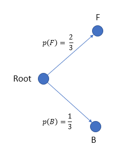
p(B) = probability of coin being biased p(F) = probability of fair coin

Since 2 fair coins,

$$ p(F)={\frac {\text {Number of fair coins}} {\text {Total number of coins}}} = \frac{2}{3}\\ p(B)={\frac {\text {Number of biased coins}} {\text {Total number of coins}}} = \frac{1}{3} $$

Note that,obviously, as output is either biased or fair coin

$$ p(F) + p(B) = \frac{2}{3} + \frac{1}{3} = 1 $$

This total probability being 1 should be satisfied from all branches of any node in the tree.

This is not yet over. A coin is picked up from 3 sets. Thus we derive one more level as follows.

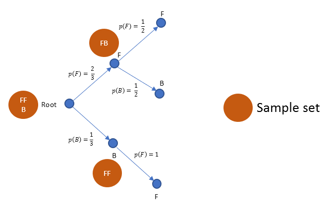
Once a coin is picked up out of "FFB" set, if picked up coin is "F", then remaining set for further possibility has only "FB". And outcome out of this remaining set could be either "F" or "B", each having equal chance, thus halved probability.

Similarly, once "B" is picked up, with remaining set containing "FF", the outcome is always only a "F" with 100% certainty. This is also depicted above as probability being 1.

Note, now we have multiple probabilities for p(F) and p(B). This is now mainly because we did not just have 2 coins to start with "FB", but "FFB", thus this additional level needed.

In same way, now we extend to the H and T possibilities of each end node. Note the p(H) and p(T) for B in particular where, heads has 2/3rd times chance of showing up.

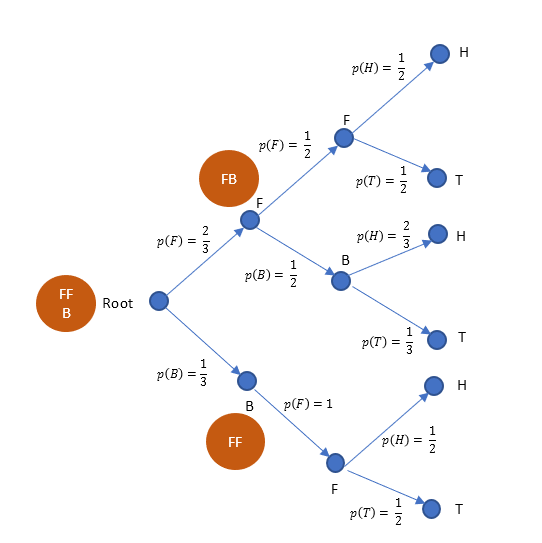
That is it. We have drawn a tree of all possible outcomes, with associated probabilities.

Note that, p (B and H) = p (H and B), both are same. That is,

p( final outcome being both biased coin with heads) = p(final outcome of heads being a biased coin).

Note that p( A and B) is not p (A | B). Both mean different, with latter being conditional probability.

From Figure 3, p (B and H) is the highlighted path, thus we multiply their probabilities in the path.

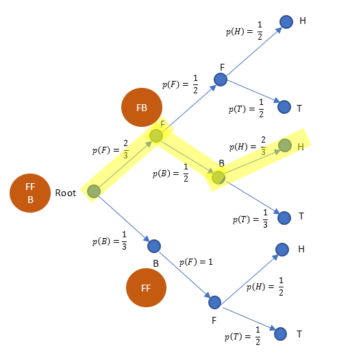
$p(\text {B and H})= \frac{2}{3}. \frac{1}{2}.\frac{2}{3} = \frac{4}{18} = \frac{2}{9}$

Recall the question, "Given that picked up coin is heads, what is the probability that the coin is biased?"

That is, given H, what is p(B). In other words, what is p(B|H)?

Notice, here the prior event is "heads" being picked up. Let us calculate all the probabilities of heads being picked up. That is p(H).

$p(\text {H})= \frac{2}{3}. \frac{1}{2}.\frac{1}{2} + \frac{2}{3}.\frac{1}{2}.\frac{2}{3} + \frac{1}{3}.1.\frac{1}{2} = \frac{2}{12} + \frac{4}{18} + \frac{1}{6} = \frac{15}{27}= \frac{5}{9}$

Coming back to p(B and H), it can be interpreted as

p( final outcome being both biased coin and heads) = p (outcome of all possible heads scenario) x p (outcome of getting biased coin, given heads has occurred).

$p(\text {B and H})= p(\text {H}) . p(\text {B} \mid \text {H})$

Re read. This is the very crux of our solution. The latter in above equation can now be readily derived.

$p(\text {B} \mid \text {H}) = \frac{p(\text {B and H})}{p(\text {H})} = \frac{2}{9} . \frac{9}{5}= \frac{2}{5}$

Thus, the probability of getting biased coin, given heads occurred is $\frac{ 2 }{ 5 }$. This conforms with Khan academy's answer as well (which is $\frac{ 4 }{ 10 }$). Note that even though I have not yet understood, why the tree (which is different) in Khan academy's video has to be balanced, I am now able to derive the same solution via a slightly different approach.

Example 2 (Udacity): Suppose there is a known statistics that 1% of population gets cancer. When we then test them, there is 90% chance, test is positive, if that person being tested has cancer. Similarly, there is also 90% chance, test is negative, if that person being tested does not have cancer. As first event, we test a person, and the result is positive. Now what is the probability that the person has cancer?

Let us assume,

p(C) = probability of cancer
p(+/C) = probability of test being +, given the person has cancer.
p(+) = probability of test being +
p(C/+) = probability of person having cancer, given the test is positive
p(C and +) = probability of person having cancer and test being positive.

Visualizing in tree diagram, just like previous problem..

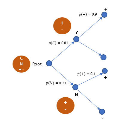
Rephrasing the question, what is the probability of person having cancer, given the test conducted on him is positive. In other words, what is p(C/+).

From the tree, we can derive the probability of person having cancer and test being positive, that is p(C and +)

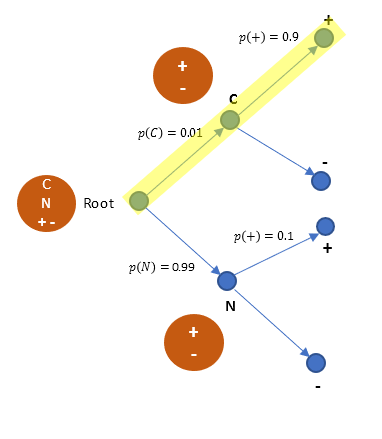
p(C and +) = (0.01) (0.9) = 0.009

From the tree, we can also derive probability of all outcomes of test being positive, that is p(+)

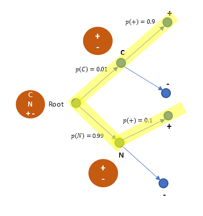
p(+) = (0.01)(0.9) + (0.99)(0.1) = 0.108

We now know from previous example,

p(C and +) = p(+) . p(C/+)

Thus,

$p(\text {C/+}) = \frac{p(\text{C and +})}{p(\text{+})}= \frac{0.009}{0.108} = 0.0833$

Thus, the probability of a person having cancer, given the test is positive, is 0.0833 or $8.3$ which also conforms with the answer in Udacity.

Summarizing, with single approach we are able to solve both cases, as intuitive as possible (hopefully), even when the methods handled in both cases by respective platforms are not fully clear.

Note: I have not yet gotten in to generalized formula and leaving that to readers'. Specifically in above examples, the denominator probability, that is p(H) in former case, or p(+) in latter case, is actually summation of those probabilities, so in strict sense, should be prefixed with a summation symbol, and index. For brevity, I stuck to the simple form. Once you start sorting out more examples with this approach, the summation and thus the intuition behind the general formula would become clearer.

General Bayes' formula with summation (inference now left to reader as food for thought):

$$ p(A_i \mid B) = \frac{p(B \mid A_i)p(A_i)}{\sum_{i=1}^n p(B \mid A_i)p(A_i)} $$